(December 2021) What I’ve been up to recently, and what I’m working on.
Published:
It’s been a while since I’ve updated my blog. I’d like to share a couple updates on what I’ve been doing, and what I hope to accomplish within the next month. I’ll start in chronological order, making note of the approximate dates when I worked on things.
Also, my laptop is acting up right now, so I can’t add links (freezes while typing every $n$ characters…). I really need a new machine, don’t I. If anyone is willing to hire me, or sponsor a new machine… of course not… right? It is Christmas, after all…
Table of Contents
- Part I: Exploration and computational experiments.
- Bayesian inference for an ion channel model
- References
- Appendix
Part I: Exploration and computational experiments.
By July 2021, I had completed my last, pre-defense committee meeting, and was fully committed on writing my thesis. However, there were several unturned stones that were bothering me, and in the absence of both intervention and calculated reasoning, I decided to spend my newfound time away from the lab in exploring these ideas. I was initially quite confident that I could complete what I wanted to do in a couple weeks. The subtext, of course, is that I didn’t, and, since none of this work will be in my thesis nor any eventual publication, I wasted several months, and continue to face the emotional, physical, and financial consequences of this series of unfortunate decisions.
Regrets aside, what did I actually accomplish in this period (roughly July through to September)?
Molecular dynamics (MD)
Introduction
By this, I mean that I used OpenMM and mostly-default CHARMM-GUI settings to perform all-atom simulations of WT and F431A HCN2 channels. The homology models were built using the SwissModel server from HCN1 (PDB: 5U6O, 5U6P, 6UQF, and 6UQG). These pilot experiments were inspired by those of the isolated segment of Kv1.5 channels shown in Labro et al. (2003). This study was interesting because it focused on the PVP hinge motif, the first proline of which is homologous to F431 in HCN2, and showed that this first proline was required for channel opening. Their MD simulations were fairly limited, at 10 ns in duration and involving only the four S6 segments. The authors suggested that the first proline in the PVP motif introduces a kink that allows the pore to dilate upon voltage-sensor activation.
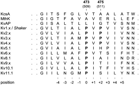
Sequence alignment of Kv channels around the *PVP* motif, showing its conservation. Figure reproduced without permission from Labro et al. (2003).
Differences between HCN and Kv channel opening mechanisms
However, the mechanism of pore opening likely differ between HCN and Kv channels. There are several reasons for this, including:
1. Different relative arrangements of the voltage-sensing domain (VSD) and pore domain (PD).
In HCN channels, VSDs interact with PDs of the same subunit, whereas in Kv channels, VSDs interact with PDs of adjacent subunits. These configurations are called ‘non-domain swapped’ and ‘domain-swapped,’ respectively.
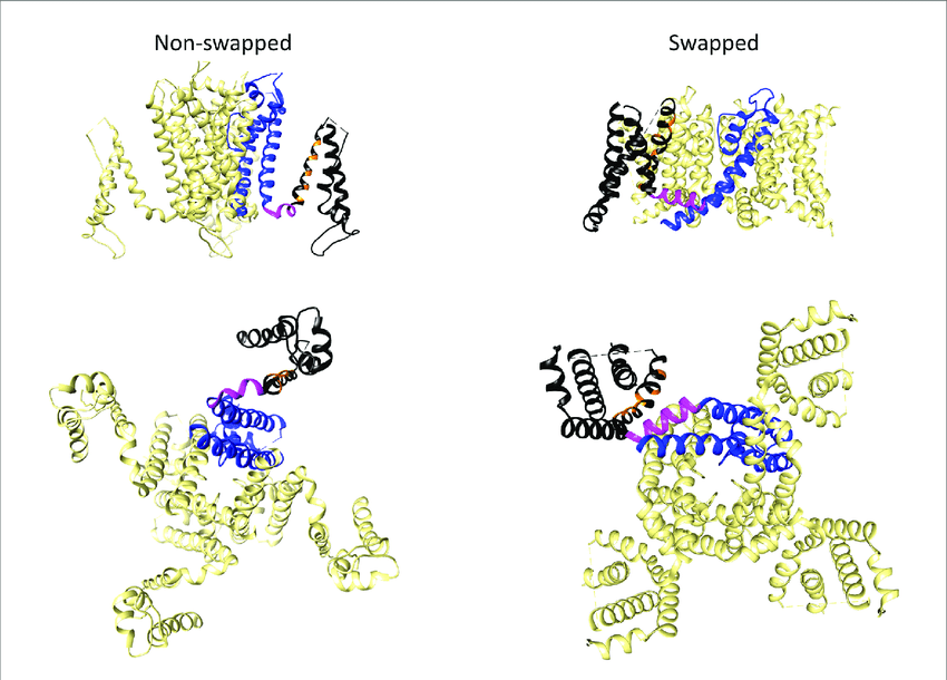
Pores are coloured blue, S4-S5 linkers in magenta, and the voltage-sensing domain (VSD) in black. Orange marks positively charged S4 residues. Views are from the membrane plane (top) and from the cytosolic side (bottom). Figure reproduced without permission from Barros et al. (2020).
2. Differences in VSD-PD (‘electromechanical’) coupling.
Due to the different structural arrangements of the PD and VSD, the mechanism by which voltage-sensing is coupled to the pore is also different. However, the most striking evidence of this is that HCN channels activate upon hyperpolarization, rather than depolarization like most Kv channels, despite HCN channels being members of the latter. In fact, gating currents also show that the S4 segments also move similarly upon changes in membrane potential (e.g. Mannikko et al. (2002), Ryu et al. (2012)).
3. Differences in opening energetics and kinetics.
The current model of HCN channel activation is that, in the depolarized state, the VSDs push the pore closed and are thus autoinhibitory for channel opening. This is supported by structures of HCN1 and HCN4 that show tight planar arrays formed by S4, S5, and S6 (Lee and MacKinnon (2017), Saponaro et al. (2021)). The next key idea comes from my Master’s lab in an alanine/valine scan of 20-odd residues in the distal S6 of HCN2. In this study, Vincenzo (‘Enzo’) Macri, a PhD alum, found that the majority of mutants exhibited compromised opening (Macri et al. (2009)). In contrast, similar studies in Shaker Kv channels showed the opposite, i.e. that most mutations in the distal pore resulted in greater opening at rest. A straightforward interpretation of these observations is that the energetics of pore opening differ between Shaker and HCN: the open state is intrinsically less favourable in Shaker, but more favourable in HCN chanels.
Hyperpolarization-dependent activation in HCN channels can therefore be explained as follows. Though the open state of the pore is energetically favoured, it cannot open upon depolarization due to autoinhibition from the VSDs, which pack against and close the pore at rest (depolarization). However, when displaced by hyperpolarization, VSD-PD contact is weakened, allowing the pore to relax into an open state. In contrast, opening of Kv channels is active and requires S4s the ‘pull’ the S6 gate open (hence, ‘electromechanical’), whereas closing is passive.
Below are some additional, noteworthy observations regarding electromechanical coupling in HCN and Kv channels.
a. Kv channels require an S4-S5 linker, but not HCN channels.
Electromechanical coupling in Kv channels requires a short, intracellular linker between the S4 and S5 (‘S4-S5 linker’), presumably to transduce the aforementioned force of ‘pulling.’ Conversely, deletion or truncation of the S4-S5 linker does not impair normal gating in HCN channels. In fact, this appears to be the case for a number of ‘non-domain swapped’ channels, including hERG and rEAG (Lorinczi et al., 2015).
b. Weak VSD-PD coupling.
VSD-PD coupling is very weak in HCN channels! For one, kinetic models have predicted allosteric coupling factors that are at least 100 times less than those of Shaker (Ryu et al. (2012), Flynn et al. (2018)). Secondly, many mutations of the S4 and S5 cause raise baseline conductance at positive voltages, or even result in constitutively open channels (e.g. Cheng et al. (2007), Wemhöner et al. (2012), Ramentol et al. (2020)). This may seem surprising, given the result of mutations in the distal S6, but actually, this actually has a very intuitive explanation.
Given the favourable energetics of pore opening, channels would be expected to open at positive voltages in the absence of either: (1) voltage-sensing or (2) VSD-PD interaction. Since VSD-PD coupling is weak and required for deactivation, but not activation, channel closing is easily compromised by relatively small perturbations. Perhaps the best demonstration of weak VSD-PD coupling is the ability to convert HCN channels into depolarization-activated channels with just a few mutations at the S4-S5 interface (Ramentol et al. (2020)).
However, there still remains a lot of work to be done. Personally, I’ve always been more interested in the kinetic side of the story, as there are a number of unique kinetic features of HCN channels. In fact, I could write another blog post about these. For example, while HCN and hERG are non-domain swapped channels that don’t require their S4-S5 linkers for normal voltage-gating, hERG not only exhibits depolarization-dependent activation, but also opens much faster than HCN2/HCN4 - less than a second and several seconds, respectively.
So, VSD-PD coupling isn’t the whole story! To explain these differences, we need to (re)-visit the S5 and S6. In recent years, we have uncovered much about how the S4 and S5 communicate, and how C-terminal regions of the channel interact with the VSD, but much remains unknown about the S6. How does it open? How does it close? I attempted to answer the latter in my Master’s thesis (I’ll add a link to it in six or so months when it’s finally published).
Results of a brief set of MD experiments
As stated above, I performed a series of MD experiments using homology models of WT and F431A HCN2 channels. As mentioned above, F431 is homologous to the first proline in the PVP hinge motif. In HCN channels, this pheylalanine is located in the distal S6 and is located across all isoforms. My Master’s thesis focused on understanding the biophysics of the F431A mutant using electrophysiology and mathematical modelling, but these methods naturally come short in providing a truly molecular interpretation.
Like Labro et al. (2003), my simulations were 10 ns long in duration (following appropriate minimization and equilibration), but whereas Labro and colleagues only simulated the S5 segments, I performed all-atom simulations in which the channels were embedded and simulated within a POPC bilayer.
For the sake of brevity (there’s still much more to cover in this blog post…), I will only show summary metrics of these experiments. I show both the summary figures and relevant (partial) code used to generate the data, but not necessarily the visualizations. All code is written in Python 3.7 and assumes the follow packages are imported, and that the trajectory is centerd and aligned:
import numpy as np
import pandas as pd
import MDAnalysis as mda

def RemoveOverallMovement(
    u: mda.Universe, u2: mda.Universe, out_path: str
):
    """Align a trajectory to its first frame to remove overall movements

    Args:
        u (mda.Universe): coordinates and trajectory
        u2 (mda.Universe): copy of `u`
        out_path (str): filename for saved alignment (dcd file)

    Returns:
        mda.Universe: aligned mda Universe
    """
    u.trajectory[-1]
    u2.trajectory[0]

    align.AlignTraj(u, u2, select='name CA', filename=out_path).run()

    return u
Root Mean Squared Deviation (RMSD)
RMSDs were computed for the entire trajectory using the backbone carbons of each residue, and then averaged across the four subunits. RMSD trajectories are often used to estimate how close to steady-state a system is: the higher the RMSD, the more ‘dynamic’ the system and the further it is from steady-state. In my simulations, RMSDs seem to stabilize, or be very close to stabilizing, by the end of 10 ns. However, the S4 segment of ‘F431A_5u6o’ seems to be substantially more dynamic than other models simulated (see legend of Figure 2 for an explanation of the naming). This could indicate that the F431A mutation, despite being located on the S6,
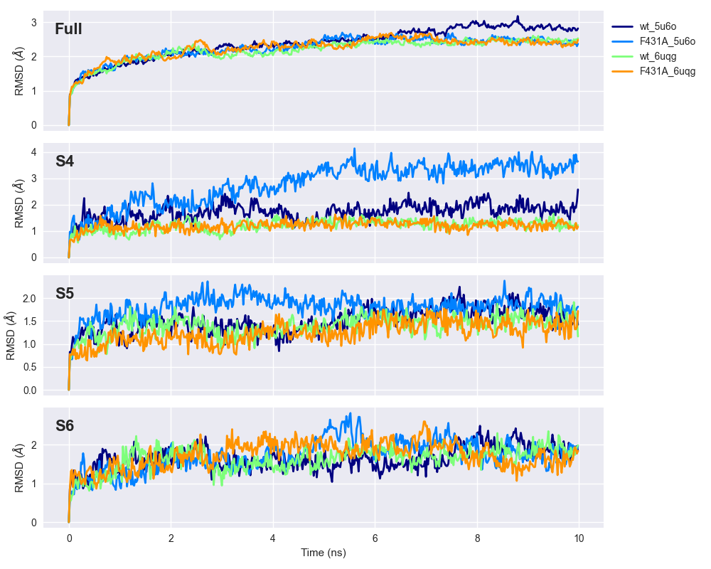
RMSD over the 10-ns trajectory is shown for the full protein ('Full') and individually for segments S4, S5, and S6. RMSD values were averaged across subunits. Colours correspond to different protein templates: WT HCN2 ('wt_5u6o' and 'wt_6uqg'), F431A HCN2 ('F431A_5u6o' and 'F431A_6uqg'). The suffices correspond to the RCSB IDs of models used as homology templates, where 5U6O corresponds to the closed HCN1 channel (Lee and MacKinnon, 2017) and 6UQG to constitutively open HCN1 mutant (Lee and MacKinnon, 2019).
def do_RMSD(u: mda.Universe, selections: list, sel_names=[], weights=None):
    """perform RMSD on each frame of u.trajectory

    Args:
        u (mda.Universe): coordinates and trajectory
        selections (list): list of strings conforming to MDAnalysis' atom selection language, e.g. 'resid 1-50'
        sel_names (list): list of strings representing names of groups in `selections` used as column headers for output dataframe. If empty, uses default numbers.
        weights (None or str, optional): weighting for RMSD calculation, of same length as number of particles in corresponding AtomGroup. Use 'mass' for weights of particle weights. Defaults to None.

    Returns:
        pd.DataFrame: RMSD values
    """
    # universe is automatically translated/centered
    R = rms.RMSD(
        u, u, select='backbone', weights=weights,
        groupselections=selections, ref_frame=0
    )

    R.run()

    # column names for output dataframe
    cols = ['Frame', 'Time (ns)']
    if len(sel_names) < 1:
        cols.extend(list(range(len(selections))))
    else:
        cols.extend(sel_names)

    return pd.DataFrame(R.rmsd, columns=cols)
Root Mean Squared Fluctuation
The RMSF is very similar to the RMSD if you imagine averaging the RMSD for each timepoint. The RMSF measures the movement of each residue throughout the trajectory. Comparing the same simulations as above, we see that the RMSFs are very similar, although ‘F431A_5u6o’ seems to be more dynamic between S4-S5 and just distal to the S6.
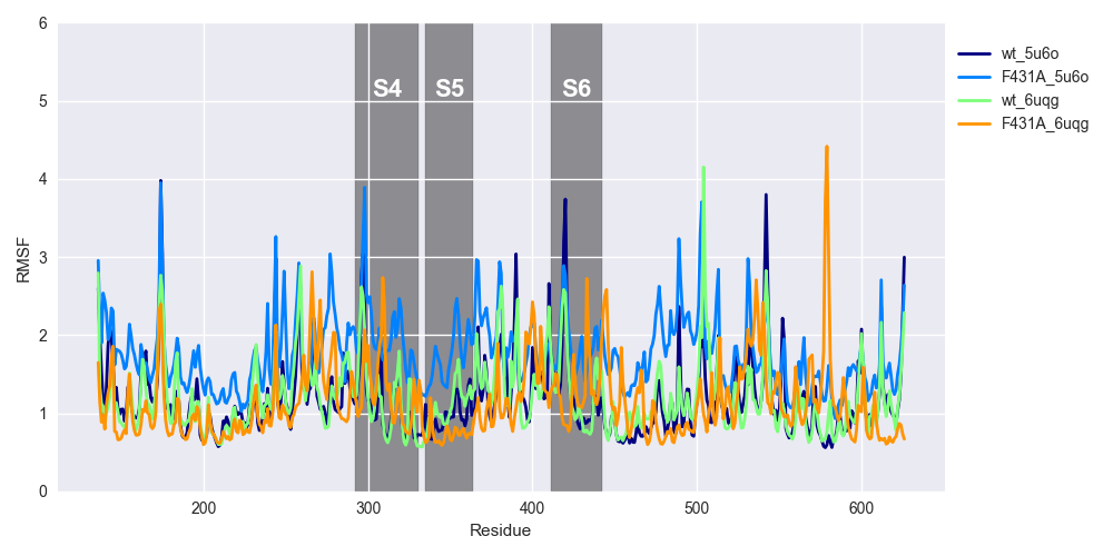
RMSFs over the 10-ns trajectory is shown for WT HCN2 ('wt_5u6o' and 'wt_6uqg') and F431A HCN2 ('F431A_5u6o' and 'F431A_6uqg'). See the legend of Figure 4 for an explanation of suffices.
def do_RMSF(
    u: mda.Universe, out_path: str,
    save_avg_pdb=False, save_avg_traj=False,
    show=True, out=False
):
    """Compute RMSF over trajectory relative to average structure

    Args:
        u (mda.Universe): coordinates and trajectory loaded with MDAnalysis
        out_path (str): folder to hold output files
        save_avg_pdb (bool, optional): whether to save average pdb. Defaults to False.
        save_avg_traj (bool, optional): whether to save average-aligned trajectory. Defaults to False.
        show (bool, optional): whether to plot RMSF. Defaults to True.
        out (bool, optional): whether to write PDB coloured by RMSF (B factors). Defaults to False.

    Returns:
        np.ndarray: 1D array of RMSF values for each frame
    """
    # create average structure
    avg = align.AverageStructure(
        u, u, select='protein and name CA', ref_frame=0
    ).run()

    if save_avg_pdb:
        avg.atoms.write(out_path + "_avg.pdb")
        print("Saved averaged PDB to %s_avg.pdb" % out_path)

    # align backbone of average structure and trajectory
    if save_avg_traj:
        align.AlignTraj(
            u, avg.universe, select='protein and name CA',
            filename = out_path + "_avg_aligned.dcd"
        ).run()
        print("Saved average-aligned trajectory to %s_avg_aligned.dcd" % out_path)
    else:
        align.AlignTraj(u, avg.universe, select='protein and name CA').run()

    # compute rmsf
    c_alphas = u.select_atoms('protein and name CA')
    R = rms.RMSF(c_alphas).run()

    if show:
        plt.plot(c_alphas.resids, R.rmsf)
        plt.xlabel('Residue number')
        plt.ylabel('RMSF ($\AA$)')
        plt.show()

    ## add empty attribute for all atoms
    if out:
        np.save(out_path + "rmsf.npy", R.rmsf)
        print("RMSF saved to %s_rmsf.npy" % out_path)

        u.add_TopologyAttr('tempfactors')
        protein = u.select_atoms('protein') # select protein atoms
        for residue, r_value in zip(protein.residues, R.rmsf):
            residue.atoms.tempfactors = r_value
        u.atoms.write(out_path + '_rmsf.pdb')
        print("RMSF-coloured PDB saved to %s_rmsf.pdb" % out_path)

    return R.rmsf
Radius of gyration (Rg)
Radius of gyration (Rg) is a familiar concept to physicists, but perhaps not for most (traditional) biologists. Wikipedia describes it as follows:
the axis of rotation is defined as the radial distance to a point which would have a moment of inertia the same as the body's actual distribution of mass, if the total mass of the body were concentrated there
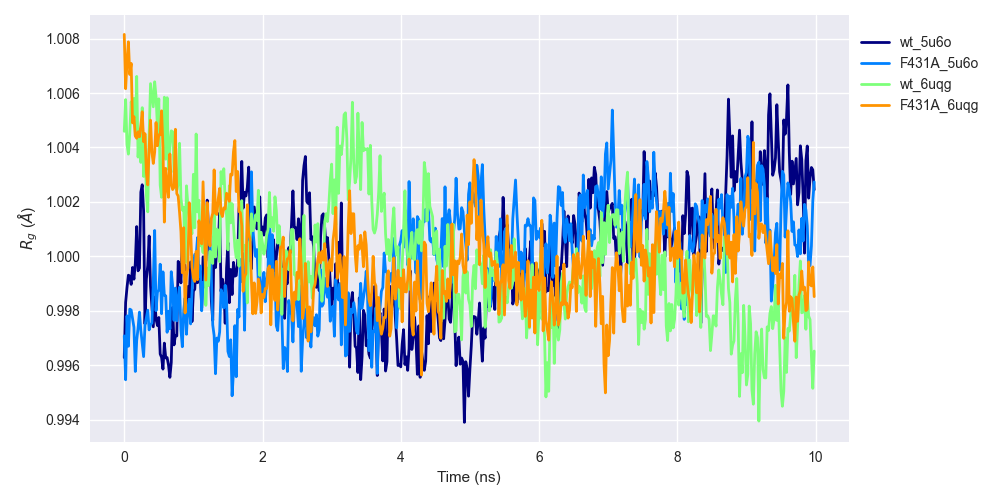
Radii of gyration over the 10-ns trajectory is shown for WT HCN2 ('wt_5u6o' and 'wt_6uqg') and F431A HCN2 ('F431A_5u6o' and 'F431A_6uqg'). See the legend of Figure 4 for an explanation of suffices. Radii of gyration were averaged over each subunit and normalized by subtracting the mean of each time series.
def do_Rg(u: mda.Universe):
    """Compute radius of gyration of backbone over trajectory

    Args:
        u (mda.Universe): coordinates and trajectory

    Returns:
        pd.DataFrame: radius of gyration with column of frames
    """
    prot = u.select_atoms('protein and backbone')

    frames = []
    Rg = []
    for ts in u.trajectory:
        Rg.append(prot.radius_of_gyration())
        frames.append(ts.frame)

    return pd.DataFrame([frames, Rg], columns=["Frame", "Rg"])
Pore diameter analysis with HOLE
The last of the “MD-specific” analyses I did was use HOLE to measure pore widths for each simulation. HOLE is an interesting program with a lot of history in the ion channel field. I don’t really know how it works, but HOLE is used extensively to compute the width of ion channel pores, which I believe are located in structures using properties such as residue size and hydrophobicity. Some more recent tools have been developed, a bunch of which are available on web servers, e.g. MOLEonline. I don’t find these tools particularly novel or innovative, but I admittedly also don’t understand them very well. Another software of this variety is the Channel Annotation Package (CHAP) which was developed by Klesse and colleagues at Oxford (Klesse et al. (2019)), although I first heard of it from Rao et al. (2019). I like CHAP, since it’s based on molecular dynamics simulations, and even tried it on my own several years ago, confirming the authors’ results on HCN Rao et al. (2019).
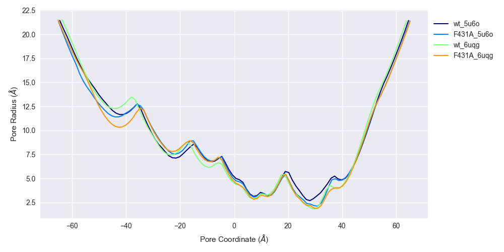
Pore profiles over the 10-ns trajectory is shown for WT HCN2 ('wt_5u6o' and 'wt_6uqg') and F431A HCN2 ('F431A_5u6o' and 'F431A_6uqg'). See the legend of Figure 4 for an explanation of suffices. The pore profiles are roughly identical, suggesting that the mutation doesn't strongly affect pore radius. Pore widths are computed using the last frame of each trajectory.
Network analyses with Cytoscape
After the initial MD analyses seemed to not give a clear indication of how F431A affected the dynamics of HCN2 channels, I turned to network-based analyses. An intuitive representation of a protein is as a graph with residues as nodes and bonds or interactions as edges. I used Cytoscape and RINalyzer to build and analyze these graphs (called ‘Residue Interaction Networks,’ or RINs for short). The motivation was fairly simple: there may be effects of the mutation that are difficult to ‘see’ from movement-based metrics (e.g. RMSD, RMSF, etc.) alone. Indeed, some groups have combined MD and network analysis to look at allosteric signaling within proteins (e.g. Fernandez-Marino et al. (2018) and Kang et al. (2020).
This is totally irrelevant, but Po Wei (“Billy”) Kang, the first author of the second paper, spoke at a meeting I attended in 2019. At the time, I was very much insulated from other ion channel researchers (still am, I guess). His presentation then was like a conversation you have during the day to which you think of a good reply hours or days after the conversation. Anyway, what I’m trying to say is that his work is superb. Somewhat reminds me of giants like Francisco Bezanilla or Clay Armstrong, but what do I know.
Continuing on from where I left off - the application of network analysis on RINs. Network science is a very interesting developed field, and a lot of the results are intuitively integrated with fields like probability, electrical engineering, and dynamical systems. However, I only looked at a small subset of network science - network centrality. Centrality metrics all try to capture how ‘important’ a given node or edge is within a network. There are many ways to calculate centrality, including the number of neighbours a node has, the number of shortest paths that traverse a node, and similar definitions for edges. I started by computing different centrality metrics for each model (e.g. ‘WT_5u6o’, ‘F431A_5u6o’, etc.) to see whether there were differences between WT and F431A. Another aside - I know that this sounds like confirmation bias. It is, sort of. But I think about it as exploratory analysis, in the sense that I don’t know much about my system (network properties of the protein) and that I have a bunch of drill bits (centrality metrics) that fit slightly differently (address different aspects of the network). So, this is more about tool selection.
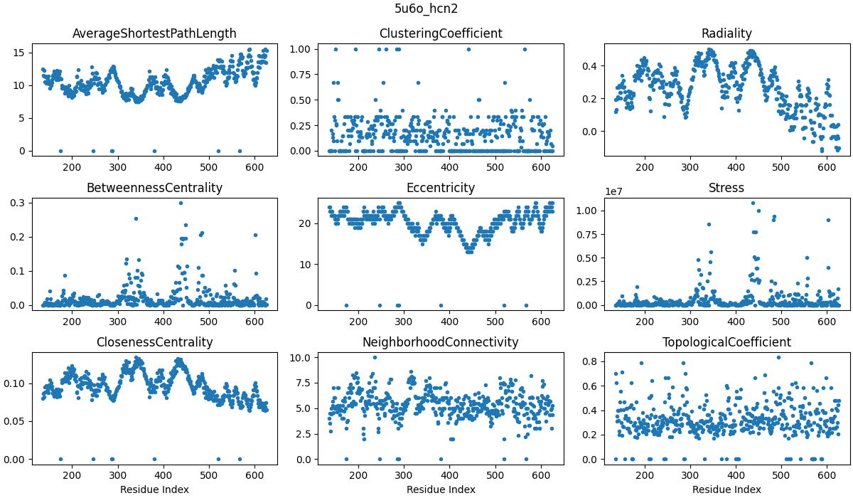
Cenrality metrics were computed for the last frame of each trajectory and averaged over subunits. Labels on the x-axis correspond to residue numbers. Explanations of each centrality measure can be found at CentiServer.
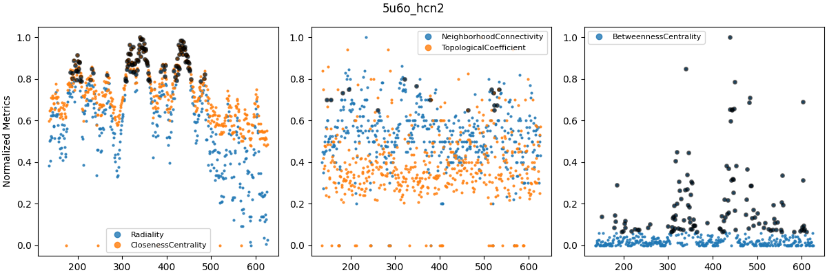
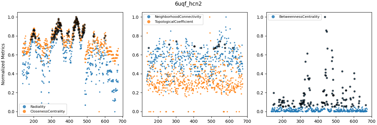
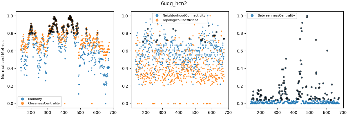
Grouped centrality metrics for WT_5u6o (top), WT_6uqf (middle) and WT_6uqg (bottom). Metrics were grouped based on apparent similarity as seen in plots such as Figure 8. Metric values were normalized in the range $[0, 1]$. Black circles indicate values in the 90th percentile.
The similarity between several centrality metrics motivated me to normalize and compare them in groups (Figure 9). However, betweenness centrality was consistently fairly different from the other metrics. Other metrics, such as clustering coefficient and eccentricity, are computed in similar ways to those in Figure 9 and were therefore not considered further (i.e. they represent similar types of information). The plots above were all for WT models, as I’ve left out analyses of F431A for brevity. However, it turns out that betweenness centrality (BC) could distinguish between F431A and WT models. In other studies, BC has been used to analyze allosteric signaling pathways (e.g. Kang et al. (2020), and this Github repo).
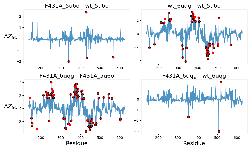
Normalized centrality values were computed for each model, and then subtracted according to the labels on top of each subplot. Normalization was done by computing Z-scores: subtracting the mean and dividing the standard deviation of each dataset. A negative difference value ($\Delta Z_{BC}$) corresponds to lower betweenness centrality in the leftward model of each subtraction. Thus, comparing F431A_5u6o and WT_5u6o, the mutation results in a loss of a central residue in the distal S6 and a significant gain in centrality for a nearby upstream residue.
Figure 10 shows differenced Z-scores of betweenness centrality between different pairs of models. The plot that stands out most to me is the top left, which shows the difference between F431A_5u6o and WT_5u6o, which were both built using a closed HCN1 channel as template. This plot shows a substantial decrease in centrality of a residue in the distal S6, and a concomitant increase in centrality of another located very closeby, but slightly higher on the S6. These residues, it turns out, are at indices 431 and 428, respectively. It seems to suggest that the loss of allosteric function in F431A is being compensated by residue 428. In fact, residue 428 is a tyrosine - another bulky, aromatic residue! Could this be a coincidence?
This brings me back to the very beginning of my Master’s thesis. I expound on this idea more in my thesis, but I essentially started off thinking that what F431 did was to mediate contact between the S5 and S6 so that packing forces from the S4 would be effectively transmitted to the pore.
Closing remarks.
That concludes most of this section. I just want to note that I felt like I learned a lot about other aspects of programming from this project, including high-performance programming for molecular dynamics simulation in OpenMM (granted, the code to do so was already laid out for me) and using a REST API (Cytoscape). See Script that interfaces with Cytoscape to generate and analyze RINs for the full script I used to automate RIN creation for dozens of protein files, analyze their networks in Cytoscape, and write outputs to .PDB and .CSV files.
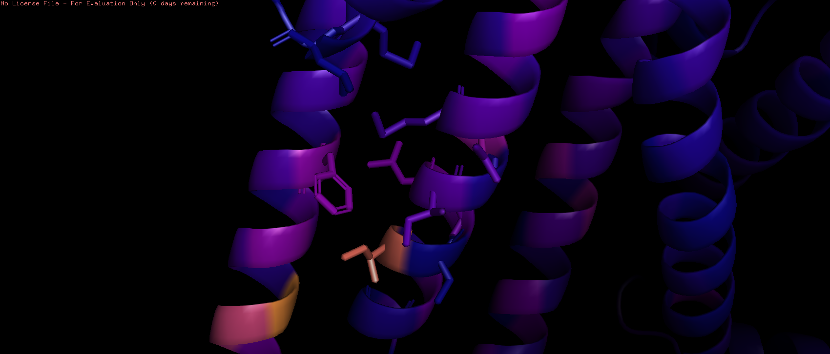
Close-up view of the C-terminal S4 (right), S5, and S6 (left) for 'WT_5u6o.' The bottom of the image corresponds to the cytosolic direction. F431 and its first neighbours are shown as sticks. Residues (of the full protein) are coloured according to their betweenness centrality, where higher values are indicated by brighter colours. Note how the majority of the protein is uniformly dark, besides residues near F431.
Bayesian inference for an ion channel model
Well. I also did some of this. But it’s 9AM Christmas morning and I haven’t slept at all, writing this post. I should probably stop here. I don’t know if or when I’ll continue this, but for now, happy holidays.
References
Barros F, de la Peña P, Domínguez P, Sierra LM, Pardo LA. The EAG Voltage-Dependent K+ Channel Subfamily: Similarities and Differences in Structural Organization and Gating. Front Pharmacol. 2020;11:411. Published 2020 Apr 15. doi:10.3389/fphar.2020.00411
Cheng L, Kinard K, Rajamani R, Sanguinetti MC. Molecular mapping of the binding site for a blocker of hyperpolarization-activated, cyclic nucleotide-modulated pacemaker channels. J Pharmacol Exp Ther. 2007;322(3):931-939. doi:10.1124/jpet.107.121467
Fernández-Mariño AI, Harpole TJ, Oelstrom K, Delemotte L, Chanda B. Gating interaction maps reveal a noncanonical electromechanical coupling mode in the Shaker K+ channel. Nat Struct Mol Biol. 2018;25(4):320-326. doi:10.1038/s41594-018-0047-3
Flynn GE, Zagotta WN. Insights into the molecular mechanism for hyperpolarization-dependent activation of HCN channels. Proc Natl Acad Sci U S A. 2018;115(34):E8086-E8095. doi:10.1073/pnas.1805596115
Kang PW, Westerlund AM, Shi J, et al. Calmodulin acts as a state-dependent switch to control a cardiac potassium channel opening. Sci Adv. 2020;6(50):eabd6798. Published 2020 Dec 11. doi:10.1126/sciadv.abd6798
Klesse G, Rao S, Sansom MSP, Tucker SJ. CHAP: A Versatile Tool for the Structural and Functional Annotation of Ion Channel Pores. J Mol Biol. 2019;431(17):3353-3365. doi:10.1016/j.jmb.2019.06.003
Labro AJ, Raes AL, Bellens I, Ottschytsch N, Snyders DJ. Gating of shaker-type channels requires the flexibility of S6 caused by prolines. J Biol Chem. 2003;278(50):50724-50731. doi:10.1074/jbc.M306097200
Lee CH, MacKinnon R. Structures of the Human HCN1 Hyperpolarization-Activated Channel. Cell. 2017;168(1-2):111-120.e11. doi:10.1016/j.cell.2016.12.023
Macri V, Nazzari H, McDonald E, Accili EA. Alanine scanning of the S6 segment reveals a unique and cAMP-sensitive association between the pore and voltage-dependent opening in HCN channels. J Biol Chem. 2009;284(23):15659-15667. doi:10.1074/jbc.M809164200
Männikkö R, Elinder F, Larsson HP. Voltage-sensing mechanism is conserved among ion channels gated by opposite voltages. Nature. 2002;419(6909):837-841. doi:10.1038/nature01038
Ramentol R, Perez ME, Larsson HP. Gating mechanism of hyperpolarization-activated HCN pacemaker channels. Nat Commun. 2020;11(1):1419. Published 2020 Mar 17. doi:10.1038/s41467-020-15233-9
Rao S, Klesse G, Lynch CI, Tucker SJ, Sansom MSP. Molecular Simulations of Hydrophobic Gating of Pentameric Ligand Gated Ion Channels: Insights into Water and Ions. J Phys Chem B. 2021;125(4):981-994. doi:10.1021/acs.jpcb.0c09285
Ryu S, Yellen G. Charge movement in gating-locked HCN channels reveals weak coupling of voltage sensors and gate. J Gen Physiol. 2012;140(5):469-479. doi:10.1085/jgp.201210850
Saponaro A, Bauer D, Giese MH, et al. Gating movements and ion permeation in HCN4 pacemaker channels. Mol Cell. 2021;81(14):2929-2943.e6. doi:10.1016/j.molcel.2021.05.033
Wemhöner K, Silbernagel N, Marzian S, et al. A leucine zipper motif essential for gating of hyperpolarization-activated channels. J Biol Chem. 2012;287(48):40150-40160. doi:10.1074/jbc.M112.378513
Appendix
Script that interfaces with Cytoscape to generate and analyze RINs
# modified based on:
# https://hal.archives-ouvertes.fr/hal-02389343/document

import requests, time, string
import urllib, glob, os, sys, json

import math
import numpy as np
import pandas as pd
import matplotlib.pyplot as plt

# commands to structureviz/chimera require encoding ASCII symbols into URL
# this is done using %-straddled integers
# e.g. chimera > select :.A === select%20%3A., where %20 = '\s', %3a = ':'
# note that '+' can be used inplace of '%20'
urlChimera = "http://localhost:1234/v1/commands/structureViz/send?command="
urlCreateRIN = "http://localhost:1234/v1/commands/structureViz/createRIN?"
RINparameters = "includeHBonds=true&ignoreWater=true&distCutoff=4.5"
urlDelete = "http://localhost:1234/v1/commands/network/delete"

def OpenPDB(path: str, s=urlChimera, t=5):
    # encode as URL
    q = urllib.parse.quote(path, safe='')
    s = s + "open%20" + q
    requests.get(s)
    time.sleep(t)

def DeleteHet(s=urlChimera):
    # delete non-protein
    requests.get(s + "delete%20%7e.protein")
    time.sleep(5)

def SelectProtein(sel: str, s=urlChimera):

    # clear selection
    if sel is None:
        sel = urllib.parse.quote("~select")
    else:
        sel = urllib.parse.quote(sel)

    requests.get(s + sel)
    time.sleep(5)

def DeleteAll(s=urlChimera):
    requests.get(s + urllib.parse.quote("delete #0"))
    time.sleep(5)

def AlignAll(N=6, s=urlChimera):
    q = urllib.parse.quote("mm #0 #1-%d show true" % N)
    requests.get(s + q)
    time.sleep(5)

class Cyto():
    def __init__(self, construct: str, pdb_path: str, out_path: str):
        """
        `pdb_path` should contain format field in file name, e.g. /{0}_output.pdb
        `out_path` should contain a format field in file name, e.g. /{0}_out.csv
        """

        self.NetNames = []
        self.PDBPaths = []
        self.c = construct

        self.methods_dict = dict(
            CCA='Closeness - CCA',
            BCA="Betweenness - BCA",
            RCA="Residue (ASPL change under removal of individual nodes) - RCA",
        )

        self.table_out_path = out_path
        self.pdb_path = pdb_path
        self.table_paths = []

    def NetworkNames(self, pdb_files: list):
        self.NetNames = []
        self.PDBPaths = []

        for f in pdb_files:
            # reeplace with Chimera compatible slashes
            self.PDBPaths.append(f.replace("/", "\\"))

            # get frame number
            fname = os.path.basename(f)[:-4].split("_")
            frame = int( [x for x in fname if 'Frame' in x][0][5:] )
            self.NetNames.append( "%s-%d" % (self.c, frame) )

    def GetFiles(self):
        # read all pdb files
        files = glob.glob(self.pdb_path.format(self.c))

        if len(files) < 1:
            raise Exception("No files found for < %s >" % self.c)
        else:
            self.NetworkNames(files)

        return self.PDBPaths

    def OpenPDBs_Chimera(self, port: int, t=10):
        self.GetFiles()

        url = "http://localhost:%d/run?command=" % port
        msg0 = "Opening... < {0} >"
        for f in self.PDBPaths:
            print(msg0.format(f))
            OpenPDB(f, s=url, t=t)

    def do_RIN(self, delete_het=False):

        self.GetFiles()

        # naming of RINs
        CreateRIN = urlCreateRIN + RINparameters + "&networkName={0}"

        # loop over models and create RINs for each
        for i in range(len(self.PDBPaths)):
            OpenPDB(self.PDBPaths[i])

            # delete non protein
            if delete_het:
                DeleteHet()

            # select i-th model
            SelectProtein("select #0")

            # construct RIN
            print("Creating %d-th RIN... %s" % (i, self.NetNames[i]))
            requests.get(CreateRIN.format(self.NetNames[i]))

            time.sleep(30)
            print("Deleting structure and continuing...")

            # deselect all
            SelectProtein(None)

            # delete all; open again later to set layout
            DeleteAll()

    def GetNetworkSUIDs(self):

        urlList = "http://localhost:1234/v1/commands/network/list"

        #gets the list of networks SUIDs
        networksList = requests.post(urlList)
        networksList = networksList.json()
        networksList = (networksList["data"]["networks"])

        return networksList

    def do_Centrality(self, method='BCA'):

        if method in self.methods_dict.keys():
            typeOfCentrality = self.methods_dict[method]
        else:
            raise Exception("%s centrality not supported.")

        #parameters
        urlSetNetwork = "http://localhost:1234/v1/commands/network/set%20current"
        urlCentrality = "http://localhost:1234/v1/commands/rinspector/centrality"

        #gets the list of networks SUIDs
        networksList = self.GetNetworkSUIDs()

        #calculates centralities for each network
        for j, i in enumerate(networksList):
            print("Computing centrality for %s (%d of %d)..." % (i, j, len(networksList)))

            #sets the network
            requests.post(urlSetNetwork, json={"network":"SUID:"+str(i)})

            #calculates centralities
            requests.post(urlCentrality, json={"analysisType": typeOfCentrality})

    def ExportTables(self, which='node', overwrite=False):
        # get list of table SUIDs
        u = "http://localhost:1234/v1/commands/table/list"

        if len(self.NetNames) < 1:
            self.NetworkNames()

        kw = dict(type=which)

        if which == 'all':
            kw['type'] = 'node'
            tablesList = requests.post(u, json=kw).json()["data"]["tables"]
            kw['type'] = 'edge'
            tablesList.extend(requests.post(u, json=kw).json()["data"]["tables"])

            TableNames = [n + " default node" for n in self.NetNames]
            TableNames.extend([n + " default edge" for n in self.NetNames])
        else:
            tablesList = requests.post(u, json=kw).json()["data"]["tables"]
            TableNames = ["%s default %s" % (n, which) for n in self.NetNames]

        # empty list
        self.table_paths = []

        u = "http://localhost:1234/v1/commands/table/export"
        N = len(TableNames)
        msg = "Successfully saved table < {0} > to: \n {1}"

        urlSetNetwork = "http://localhost:1234/v1/commands/network/set%20current"
        networksList = [str(x) for x in self.GetNetworkSUIDs()]
        N_networks = len(networksList)

        for i, T in enumerate(TableNames):
            print("%d-th table of %d" % (i+1, N))

            kw = dict(
                options = "CSV", table = T,
                outputFile = self.table_out_path.format(T),
            )
            # print(kw)

            if os.path.isfile(kw["outputFile"]) and (not overwrite):
                self.table_paths.append( kw["outputFile"] )
                continue

            #sets the network
            if i >= N_networks:
                kw = {"network":"SUID:" + networksList[i - N_networks]}
            else:
                kw = {"network":"SUID:" + networksList[i]}

            r = requests.post(urlSetNetwork, json=kw)
            time.sleep(5)

            r = requests.post(u, json=kw)
            time.sleep(20)

            if r.status_code == 404:
                try: print(r.json())
                except: print(r.text)
                # continue
            else:
                self.table_paths.append( kw["outputFile"] )
                print(msg.format(T, kw["outputFile"]))

        print("Saved files: \n", self.table_paths)

    def read_data(self, cols=["RINalyzerResidue", "Z-score_BCA"]):
        files = self.table_paths

        # check that files exist
        for f in files:
            if not os.path.isfile(f):
                print("Table not saved for: \n", f)

        df_lis = []
        for f in files:
            df = pd.read_csv(f, index_col=None, header=0)
            df = df.loc[:, cols].set_index(cols[0]).sort_index()
            df_lis.append(df)

        df_merge = pd.concat(df_lis, axis=1)
        return df_merge

    def analyze_bca(self, start=136, save=True, show=True):
        df = self.read_data(cols=['RINalyzerResidue', 'Z-score_BCA'])
        df_bca = pd.DataFrame([df.mean(axis=1), df.sem(axis=1)]).T

        ResIndex = np.unique([int(s.split(":")[1]) for s in df_bca.index])
        inds = list(range(0, 5*ResIndex.shape[0], ResIndex.shape[0]))

        if min(ResIndex) != start:
            ResIndex += start

        data = []

        cmap = plt.cm.get_cmap("gist_rainbow")
        chains = ['A', 'B', 'C', 'D']
        for i, x in enumerate(chains):
            clr = cmap(i/4)
            a, b = inds[i:i+2]

            y = df_bca.iloc[a:b, :]

            plt.fill_between(
                ResIndex, y.iloc[:,0] - y.iloc[:,1],
                y.iloc[:,0] + y.iloc[:,1], lw=1, label=x,
                color=clr, alpha=0.3, zorder=1
            )

            data.append(y.reset_index(drop=True))

        outp = self.table_out_path.format(self.c + "_AvgBCA")
        if save:
            df_out = pd.concat(data, axis=1)

            cols = list(range(df_out.shape[1]))
            cols[::2] = [chain + "_Mean" for chain in chains]
            cols[1::2] = [chain + "_SEM" for chain in chains]
            df_out.columns = cols

            df_out.index = df_bca.index[:df_out.shape[0]]
            df_out.to_parquet(outp[:-4] + ".parquet")

            print("Saved averaged BCA to < %s >" % outp)

        if show:

            plt.ylim([-1, 6])
            plt.xlabel("Residue")
            plt.ylabel("Betweenness Centrality")

            plt.legend()
            plt.tight_layout()
            plt.savefig(outp[:-4] + ".png")

            plt.show()

        plt.close()

        return df_bca

    def FullCentrality(self):
        self.do_RIN()
        self.do_Centrality()
        self.ExportTables()
        self.analyze_bca()

    def multi_bca(self, models: list, start=136, cmap=plt.cm.get_cmap('tab10')):

        n_models =  len(models)
        _, ax = plt.subplots(2, 2, figsize=(10, 6))
        # ax.set_xlabel("Residue", fontsize=14)
        # ax.set_ylabel("Betweenness Centrality", fontsize=14)

        df_list = []

        for i, m in enumerate(models):
            p = self.table_out_path.format(m + "_AvgBCA")
            df = pd.read_parquet( p[:-4] + ".parquet" )
            df = df.iloc[:, ::2].mean(axis=1)

            ResIndex = np.unique([int(s.split(":")[1]) for s in df.index])

            if min(ResIndex) != start:
                ResIndex += start

            df.index = ResIndex
            df_list.append(df)

        lab = "{0} - {1}"
        kw = dict(lw=1.5, alpha=0.8, label="", zorder=2)
        kw2 = dict(marker='o', ms=6, mec='k', mew=1, ls='none', zorder=3, c='r', label="")
        for i in range(0, n_models, 2):
            j = int(i/2)

            # [0,0] = wt x fa_5u6o, [1,1] = wt x fa_6uqg
            ax[j,j].set_title( lab.format(models[i+1], models[i]), fontsize=16 )
            y = df_list[i+1] - df_list[i]
            ax[j, j].plot(y, **kw)

            y = y[y.abs() >= 1.5]
            ax[j, j].plot(y, **kw2)

            # [0,1] = wt_5u6o x wt_6uqg, [1,0] = fa_6uqg x fa_5u6o
            if i > 1:
                ax[1,0].set_title( lab.format(models[i+1], models[i-1]), fontsize=16 )
                y = df_list[i+1] - df_list[i-1]
                ax[1, 0].plot(y, **kw)

                y = y[y.abs() >= 1.5]
                ax[1,0].plot(y, **kw2)

            else:
                ax[0,1].set_title( lab.format(models[i+2], models[i]), fontsize=16 )
                y = df_list[i+2] - df_list[i]
                ax[0, 1].plot(y, **kw)

                y = y[y.abs() >= 1.5]
                ax[0,1].plot(y, **kw2)

        for i in range(2):
            ax[i, 0].set_ylabel(r"$\Delta Z_{BC}$", rotation=0,
                                labelpad=16, va='center', fontsize=16)
            ax[1, i].set_xlabel("Residue", fontsize=16)

        plt.tight_layout()
        f = self.table_out_path.format("DeltaAvgBCA")
        plt.savefig(f[:-4] + ".png")
        plt.show()

models = ["wt_5u6o", "F431A_5u6o", "wt_6uqg", "F431A_6uqg"]
outp = "path/to/save/centrality/data/{0}.csv"
pdb = "path/to/save/pdb/{0}.pdb"

NetNames = ['{0}-349', '{0}-374', '{0}-399', '{0}-424', '{0}-449', '{0}-474', '{0}-499']
for m in models[3:]:
    rin = Cyto(m, out_path=outp, pdb_path=pdbp)
    rin.NetNames = [s.format(m) for s in NetNames]

    # use port 5492
    rin.OpenPDBs_Chimera(5492)

    # compute centrality
    rin.FullCentrality()

    # plot (delta) betweenness centrality z-scores
    rin.multi_bca(models)
