2021: January, February, March

First post of 2021. Updates on what I’ve been doing for the first quarter of the year, some superficial thoughts on lab things, and an outlook for the near future.

1. Thoughts on model calibration.

Recently, I’ve returned to thinking more about the issue of parameter identifiability in kinetic models of ion channels, which is intrinsically tied to problem of protocol design. I think the Mirams’ group’s work is very educational on this topic, and I’ve probably shared at least one or two of their publications here before. For those who are unfamiliar, they’ve cleanly laid out an intuitive approach to model calibration: (1) data collection, (2) global optimization, (3) exploration of the posterior distribution. I’ll try my best here to dive into each of these steps.

First, data collection in this field involves electrophysiological recordings in cell lines transfected - stably or transiently - with an ion channel of interest. Alternatively, Xenopus laevis oocytes are also commonly used as expression systems. For cell lines, the most common form of electrophysiology is patch-clamp in the voltage-clamped, whole-cell configuration. Briefly, experimenters (or nowadays, a robot) insert an electrode, enclosed within a glass ‘pipette,’ into a cell to record the electrical currents flowing across the membrane. The electrode is connected to an amplifier, which constantly computes and injects the amount of current needed to maintain the cell’s membrane potential at a level specified by the experimenter. The sequence of specified voltages used in such an experiment is known as the voltage protocol.

When kinetic modelling is desired, there are several important considerations in making a voltage protocol. These must also be balanced with the practical and experimental limitations. Two important components of a protocol are leak subtraction and conductance estimation. While there are other methods for leak subtraction (e.g. P/N subtraction),

The main contributors to leak currents are currents through a ‘leaky’ seal between the pipette and cell membrane, as well as endogenous conductances of the cell. Most experiments use cells with minimal, or otherwise blocked, endogenous conductances. Secondly, leak currents between the pipette and membrane are typically linear in amplitude with respect to voltage. Consequently, leak currents are commonly assumed to be linear. I personally start my protocols with a symmetric voltage ramp between potentials where the transfected channels are not expected to be open. If the leak is linear, then the voltage ramps can be fit by a linear equation, which can then be used to subtract the leak from the entire recording.

The second important aspect of a protocol is conductance estimation. However, it’s not as if all models incorporate conductance per se. Rather, many modelling papers in this field don’t fit physical currents. The output of a model is a vector of probabilities for each state of the model, for a given protocol. Ion channels conduct currents when open, so electrophysiological data is represented as the sum of open states in the model - that is, total open probability (this means that we are working with a kind of partially observed Markov process, or POMP, also known as a hidden Markov model, or HMM; LOTS of literature on these out there for the interested). So, where does conductance come into play? Well, ion channels can be thought of as electrical batteries with an internal resistance (inverse of conductance) and driving force. The current across a channel is then given by

This equation uses the model output ($P_o$) and conductance ($\gamma$) to, assuming the reversal potential $E_{rev}$ is known, fit the recorded currents directly. However, this is typically not done. Instead, many papers ‘normalize’ the data into the [0, 1] range and fit the model directly this way. Alternatively, the conductance approach is emulated by scaling model output to match the amplitudes of recorded currents. This is identical to estimating a conductance value, but is different in the sense that the value of the scaling factor may not be based on the observed data. One way to inform the estimation of conductance is by extrapolating from the current elicited at a maximally-activating voltage. Ideally, $P_o$ would saturate during such a step, allowing an estimation of conductance. This is also important in the normalization approach, because it locates where $P_o$ is maximal, or nearly so.

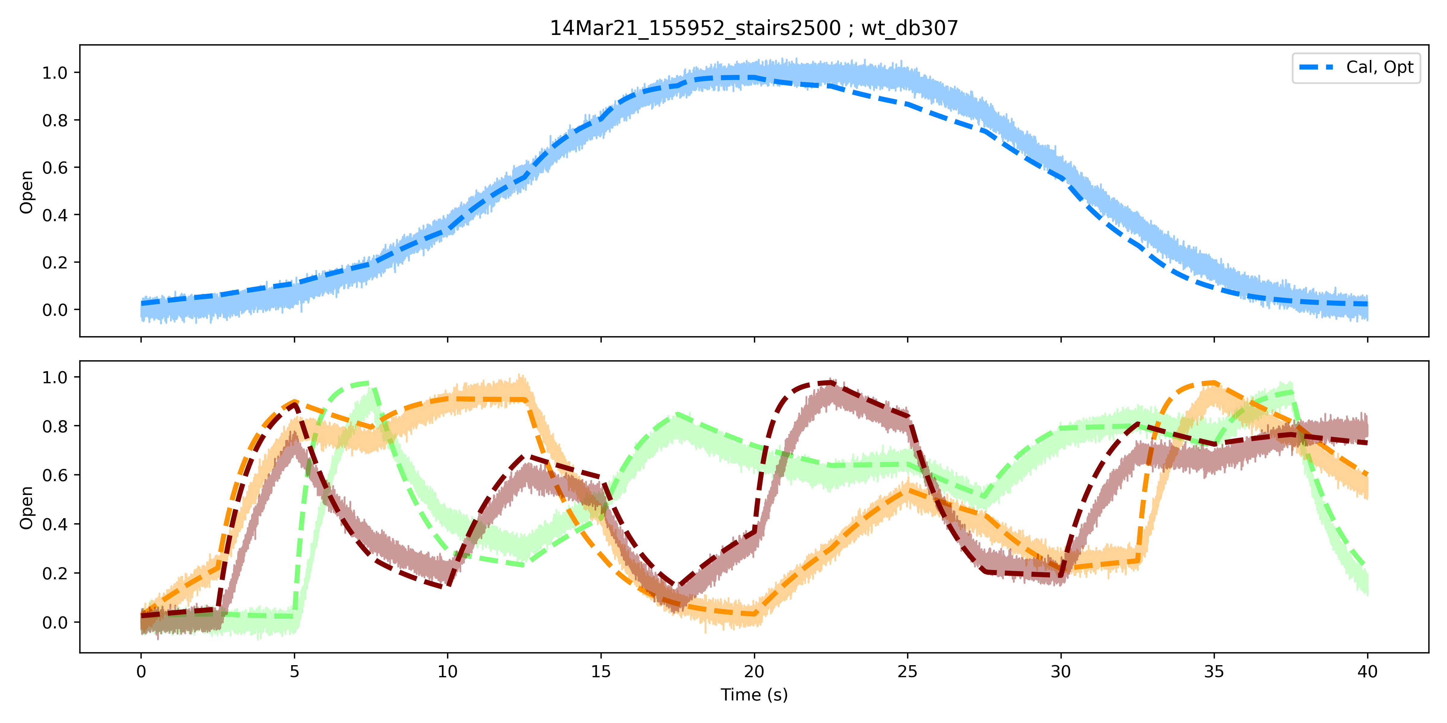
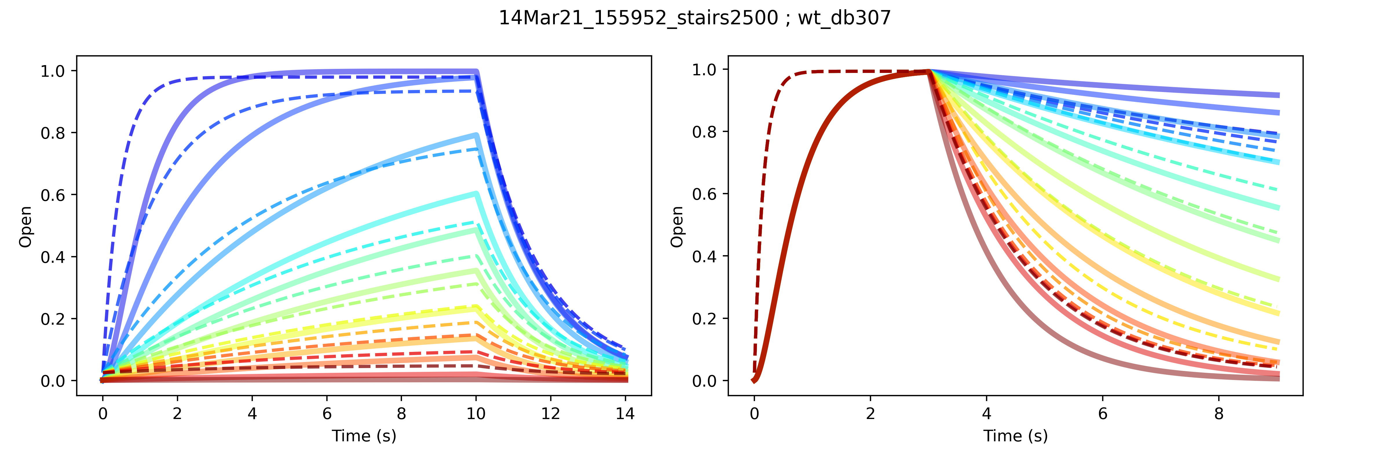
With these out of the way, let’s finally move on to the more interesting bit. Leak subtraction helps isolate channel-specific currents, while conductance estimation ensures we observe maximally-activated currents. The job of the rest of the protcol is therefore to help us traverse as much of the state space as possible, so as to maximally inform model calibration. A paper came out several years ago detailing the efficacy of using short, sinusoidal protocols to calibrate models of hERG channels expressed in CHO cells. Impressive as this, and related subsequent work, was, I haven’t found the appraoch overly useful for mammalian HCN channels, particularly because the latter are so slow in activating. Due to their slow kinetics, voltage protocols that can fit ‘short’ protocols fail to reproduce behaviour observed over slightly longer timescales at a given voltage. Here’s one example, using synthetic data:

Calibration and validation of a kinetic model using synthetic data generated from a non-traditional protocol. Top: Fit of the data used for calibration. The ‘ramp’ protocol consists of a sequence of equal-duration voltage steps that increase negatively, then positively in voltage. The calibrated model is shown in dashed lines, while the data is shown in solid, faded lines. Bottom: Fit of the calibrated model to ‘validation’ data. Three validation datasets were generated by randomly rearranging the voltage steps used in the ramp (calibration) protocol. Colours correspond to individual datasets or simulations of the calibrated model.

A model calibrated with a non-traditional protocol fails to predict synthetic data generated from traditional protocols. Traditional protocols that assess the voltage-dependence of channel activation (left) and deactivation (right) are shown with model fits and synthetic data in dashed and solid lines, respectively, in corresponding colours representing different test voltages.

Of course, I will be exploring this further, because it’s highly desirable to be able to comprehensively predict kinetics in less time. The example above represents only one particular attempt at fitting, but for the record, while the fitting algorithm did not converge, the resulting parameter values were very different from the true parameters used to generate the synthetic data. So, some issues with non-identifiability when calibrating with the chosen protocol.**

2. Interesting readings/resources.

In light of all of this modelling stuff, I’ve come across some very interesting resources. First, QuantEcon.jl has a great series of notebooks on some very pertinent topics: auto-differentiation, Markov chains, particle filters, and more. The focus is on economics, as the name suggests, but the concepts are very widespread. Secondly, I’ve starred a couple of interesting Github packages, mainly for MCMC-related business. One of these is ZigZagBoomerang.jl, which seems to be a very accessible package for this novel class of MCMC algorithms. I just found a well-written introduction and resource page on this topic, which I recommend checking out. The tl;dr is that the ZigZag and Boomerang MCMC algorithms are known as “Piecewise Determinant,” and are characterized by continuous dynamics with random changes in velocity. This supposedly helps deal with large datasets. Well, I think my own research will probably stick with either Metropolis-Hastings or, if I can get it working, Hamiltonian MCMC. Nevertheless, the visuals and names of these algorithms are eye-catching, to say the least, and probably warrant at least some exploration, given how accessible the implementations are.

Next, I, much like millions of others my age, have recently been interested in finance. Taking this recent interest with another recent interest, Bayesian statistics, together led me to the world of quantitative finance. However, I’m truly a novice in this area, so I honestly have nothing to really say about it, other than I think that there’s a lot of intriguing concepts and applications. In particular, I found a couple Github packages that I think would be worth looking into and learning from:

• Awesome multi-language compilation of resources
• PyPortfolioOpt (portfolio optimization)
• eiten (portfolio optimization)
• mlfinlab (portfolio optimization)
• DeepDow (forecasting + optimization, but not active trading)

All of the individual packages linked above are in Python! Not as many fleshed-out packages in Julia yet, unfortunately, but it’s probably only a matter of time. I would personally like to see Julia supported on Colab and Kaggle. Doing so would probably greatly boost interest in the language.