In this post, I will write about my experience working with custom voltage protocols. I will focus on how I create the protocol files for measurement in Clampex, and how I analyze the resulting recordings.

Table of Contents

• Table of Contents
• Introduction to Voltage Protocols
  • Limitations of Common Protocol Design
• Protocol Creation
  • Creating the ATF file
    • Bug warning!
    • Some more examples.
  • Final Touches.
• Analysis
  • Automated Epoch Detection.
• Conclusion

Introduction to Voltage Protocols

The most common electrophysiology hardware systems are made by Axon Instruments and HEKA Instruments. Both come with proprietary acquisition and analysis software that are jam packed with features. In voltage clamp experiments, a sequence of voltage steps, called a voltage protocol, is applied, and the resulting electrical currents are recorded. The steps of a protocol are usually of three varieties: (1) a flat pulse, (2) a linear ramp, or (3) a ‘train’ of pulses with some specified frequency. In each, duration and/or voltage can be specified during protocol creation. As such, each step, or epoch, of a protocol does not change its type, but the protocol can be repeated for several iterations (sweeps) where the duration(s) and/or voltage(s) of one or more steps change.

To summarize some relevant terminology:

• Protocol: a pre-defined time course of voltages, in a voltage-clamp experiment, that is applied to the system being recorded. When constructed using common proprietary software, protocols consist of discrete epochs which can have multiple types, durations, and voltages.
• Epoch: a single step in a protocol which has a specific type, duration, and voltage. When a protocol is repeated, the duration and voltage, but not the type, of a given epoch may change.
• Sweep: an iteration of a protocol with epochs of different durations and/or voltages. When a protocol consists of more than one sweep, there is a short period of time between the end of one sweep and the beginning of the next known as the inter-sweep interval.
• Pre-trigger length: an automatically specified, unchangeable interval at the start of each sweep that precedes the onset of the first epoch.

Limitations of Common Protocol Design

There are several unavoidable limitations when using pClamp (Axon Instruemnts) or Patch Master (HEKA) to design voltage protocols. Importantly, the number of steps in each sweep of a protocol is typically limited to around 10 or so. Consequently, these software cannot be used to create complex waveforms such as membrane potentials recorded from live cells (this is sometimes called ‘action potential clamp’) and computationally optimized protocols. However, even if you’re not doing anything particularly fancy, but just want to implement best-practices for protocol design (e.g. leak ramps, reversal ramps, membrane test steps), you can still run out of space in the protocol designer. I ran into both of these issues, so I decided to look into how to create custom protocols for use in Clampex (Axon Instruments).

Protocol Creation

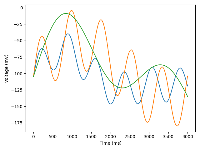
Using Python, it’s fairly straightforward to create a custom protocol. Briefly, all you need to do is to prepare your protocol as a Numpy array. For example, let’s create a sinusoidal protocol that contains three sweeps.

import matplotlib.pyplot as plt 
import numpy as np 

def sine_(A, x, t, C=-35.0):
    return A * np.sin(x/t) + C 

def create_protocol(show=False, save=None):
    # seed RNG
    np.random.seed(1337)
    # random amplitudes
    A = 100*np.random.rand(9)
    # random frequencies 
    F = 1000*np.random.rand(9)

    t = np.arange(0, 4000, 0.5)
    sines = [t]

    sines.extend([
        np.sum([sine_(A[i + 2*j], t, F[i + 2*j]) for i in range(3)], axis=0) for j in range(3)
    ])

    if show:
        for s in sines[1:]:
            plt.plot(t, s)
        plt.ylabel("Voltage (mV)")
        plt.xlabel("Time (ms)")
        plt.tight_layout()
        plt.show()
    
    if save:
        sines = np.vstack(sines).T
        print(sines.shape)
        
        np.savetxt(save, sines, delimiter=",")

create_protocol(show=True, save="...")

When we run the code above, we can see what our voltage protocol looks like.

Next, we get the protocol ready in a single array of size T x (N + 1), where T is the number of timepoints, and N is the number of sweeps. The first column contains the timepoints of measurement, while subsequent columns contain corresponding voltages. Finally, we save this array to a CSV file.

Creating the ATF file

This is a separate (sub)-section because I think it’s so cool, and because it’s only possible due to somebody else’s work (Scott W Harden). Broadly,

1. Read the CSV file that we created above
2. Create an appropriate ‘header’ for the ATF file
3. Parse each row of the CSV file as a single string, yielding the entire CSV file as one, large string

We can read the CSV file using any method. I prefer using pd.read_csv, and then converting this to an array by calling .values on the resulting DataFrame.

import pandas as pd 

# path to saved CSV file 
filename = "..."
df_data = pd.read_csv(filename, header=0).to_numpy()

ATF files contain a header that specifies information about the recording, such as sampling frequency, the number of sweeps, and the mode of stimulation. An example is shown below, assuming df_data is our custom protocol:

def default_header():
    
    ATF_HEADER="""
    ATF	1.0
    8	NUMBER_OF_SWEEPS
    "AcquisitionMode=Episodic Stimulation"
    "Comment="
    "YTop=200"
    "YBottom=-200"
    "SyncTimeUnits=20"
    "SweepStartTimesMS=0.000"
    "SignalsExported=IN 0   OUT 0"
    "Signals="	"IN 0"
    "Time (s)"
    """.strip()
    
    return ATF_HEADER

def make_header(df_data):
    """
    Create ATF header with appropriate number of sweeps and column labels  
    Returns string containing ATF header 
    """
    ATF_HEADER = default_header()
    head = ATF_HEADER.replace("NUMBER_OF_SWEEPS", 
                                str(df_data.shape[1]-1))
        
    for i in range(1, df_data.shape[1]):
        head += "\t" + """	"Trace #{i}" """"".format(i=i).strip()
    
    return head

# head = make_header(df_data)

Next, we go through the protocol row-by-row, converting each row into a string, and then appending the string to our header above. The final string can then be written to an .ATF file using basic Python.

def make_row(t, row):
    """
    Convert single `row` of data into string format for .ATF file. 
    `t` = time (index of row divided by sampling frequency) 
        
    Returns string `s` representing respective row in ATF file 
    """
    s = "\n%0.5f" % t 
    for v in row[1:]:
        s += "\t%0.5f" % v
    
    return s 

def create_atf(filename=r"./output.atf"):
    """
    Save a stimulus waveform array as an ATF 1.0 file with filename `filename`
    """
    # create ATF header 
    header = make_header()
    
    # instantiate output string, beginning with ATF header 
    # data for each trace and tiempoint will be added as newlines (rows) 
    out = header
    
    # sampling frequency
    rate = 1000/(df_data[1,0] - df_data[0,0])
    print(" The sampling frequency is %.0f kHz" % rate)
    
    for i, val in enumerate(df_data):
        out += make_row(i/rate, val)
        
    with open(filename,'w') as f:
        f.write(out)
        print("wrote", filename)

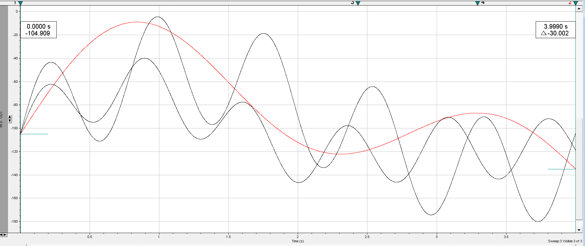
While you don’t need to necessarily save the Numpy array to a CSV file to create an ATF out of it, I find that it helps to do so for downstream analysis, which I’ll get into below. First, let’s see what the ATF file looks like when we open it in ClampFit (Axon Instruments).

Bug warning!

So, although I’ve managed to make several protocols in the past using the code above, I recently tried it with the example in this post, and found that I needed to add an additional column to the data df_data before parsing it into a single string. Otherwise, even though the ATF header contains the right information (number of sweeps), the resulting file will only contain N-1 sweeps, where the last sweep isn’t saved. Here’s the fix I used to do this:

df_data = pd.read_csv(protocol_path, header=0)
df_data.insert(df_data.shape[1], df_data.shape[1], 0.)
df_data = df_data.values 

Where, I simply added a column of zeros to the end of df_data. The rest of the procedure worked fine.

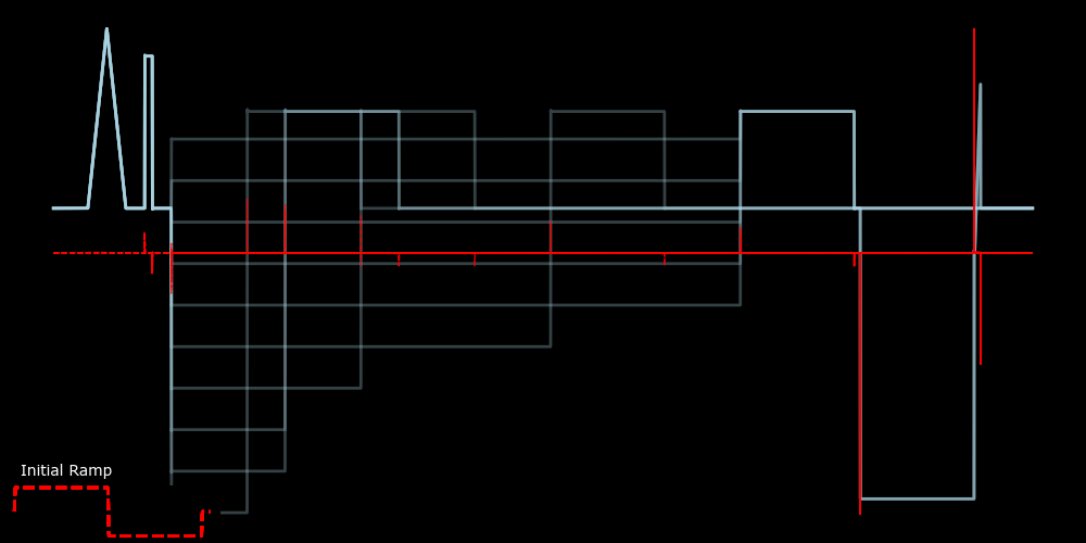
Some more examples.

Here are a couple more examples of protocols I’ve created using this method. Again, these all open in ClampFit or Clampex just fine, and can be used in recording just like any other protocol.

Final Touches.

When an ATF file is created for a custom waveform, it’s best to load it into your acquisition software (ClampEx version 8 for me) to make sure it can load properly, and if it does, save it as a protocol file (.pro). Note that .pro is distinct from .atf: the former is specifically used in acquisition, whereas the latter is a general format for data storage in the pClamp ecosystem.

Besides this, there are some additional considerations to check off before using these in an experiment:

1. The sampling frequency is set when we made the initial Numpy array. In the first example of three sinusoidal sweeps, I used a timestep of 0.5ms, which corresponds to a sampling frequency of 2 kHz. So, check that the sampling frequency is what’s expected (it can vary, for instance, depending on default settings, or the sampling frequency of your last-used protocol).

2. The inter-sweep interval and holding potential are two parameters that you will need to specify manually in Clampex. If you don’t, you might end up using defaults, which I believe are ‘Minimum’ (the minimum possible inter-sweep interval) and 0 mV, respectively.

3. While the pre-trigger length is unavoidable, you still need to account for this in your protocol! In my first example, I haven’t done this, but usually what I would do is add a flat pulse at the holding potential for about 500 ms at the beginning of each sweep. Your mileage may vary.

With this, the protocol should be ready to use for recording!

Analysis

Analysis is a bit tricky, primarily because, unlike standard protocols, custom protocols aren’t parsed by the acquisition software in terms of discrete epochs. Furthermore, it seems to be a coinflip whether or not the stimulus waveform is saved at all alongside the measured current. Regardless, because information on epochs is unavailable for custom protocols - as they weren’t made in the acquisition software - having the stimulus waveform and recorded currents in the same .ABF output file is not a huge issue.

Instead, not knowing the epochs is a bigger problem. Knowing the epochs is tremendously beneficial during analysis because it allows us to compartmentalize the data/protocol into discrete functional segments. To obtain the epochs, we can either have information about the epochs prepared in a separate file, ready for analysis, or try and automatically detect the types, levels, and durations of epochs from the voltage protocol itself. In the first method, we would simply create some data structure to hold epoch information during protocol creation, and then save it into a CSV file. Here, I’ll talk a little bit about the second method, and share some pseudo-code as well.

Automated Epoch Detection.

Let’s assume that we have a custom protocol pro.csv that contains the stimulus waveform for some recording, and we don’t know whether the recording contains the stimulus waveform. So, we prepare the following: the protocol as a pandas DataFrame, and then decide whether we need to detect epochs.

import pandas as pd 
import os 

def FindCustomEpochs(data, pname, fname, pdir=".."):
  """
  data = dataframe containing time, current, and possible voltage columns
  pname = protocol name 
  fname = filename (of original .abf recording)
  pdir = directory to protocol CSV files 
  """

  # path to protocol, if it exists
  ppath = pdir + "%s.csv" % pname
  # path to corresponding epochs, if it exists
  epath = pdir + "%s_epochs.csv" % pname 

  if os.path.isfile(ppath):
    pro = pd.read_csv(ppath, index_col=0, header=None)

    # check if we have epochs 
    if os.path.isfile(epath):
      epochs = pd.read_csv(epath, index_col=0, header=0)
      epochs = ExtractEpochs(epochs)
    else:
      # we don't have epochs available, so we need to detect them automatically
      epochs = GenerateEpochs(pro, epath)

  return epochs

ExtractEpochs simply extracts epochs from a CSV file. How it works depends on how you saved the epochs, so I won’t get into it too deeply besides saying that the output of ExtractEpochs, and indeed, GenerateEpochs, will be three dictionaries corresponding to the onset times, voltages, and types for each epoch, for each sweep.

def ExtractEpochs(df):
  """
  df = DataFrame containing information on epochs for each sweep, with columns arranged as follows:
    Times_1, Voltages_1, Types_1, Times_2, etc. 
    Where, the final number indicates sweep numbers. Therefore, for a protocol of N sweeps, there will be 3*N columns.
    There is no requirement for a uniform number of epochs (rows) for all sweeps, so some rows may be NaN.
  """
  EpochTimes = {}
  EpochLevels = {}
  EpochTypes = {}

  N = int(df.shape[1]/2)
  for i in range(N):
    # parse the columns of `df` and updates the respective dictionaries 

  return EpochTimes, EpochLevels, EpochTypes

GenerateEpochs is a function that automatically returns dictionaries EpochTimes, EpochLevels, and EpochTypes, which have sweep numbers as keys and the corresponding values for epochs in the respective sweeps as elements. For instance,

EpochTimes = {0 : [100, 200, 300], 1: [100, 200, 300]}
EpochLevels = {0: [-30, 0, -100], 1: [-30, 0, -140]}
EpochTypes = {0: ['Step']*3, 1: ['Step]*3 }

The general approach for detecting epochs is to take the first time derivative of the voltage protocol pro, and then analyze the non-zero values. Due to numerical issues, the transition between epochs may not happen at perfect, discrete transitions. Although this is desired, this is also not the case in experiments, either, so I guess this conflates with factors such as series resistance in modifying the voltage command. However, deviations due to protocol creation are expected to be far smaller in magnitude compared to experimental sources of error.

def GenerateEpochs(pro)
  """
  pro = dataframe containing voltage protocol, with timepoints in the index 
  """
  # time between measurements 
  ms = pro.index[1] - pro.index[0]
  
  # reset the index
  pro.reset_index(drop=True, inplace=True)
  # convert to numpy array 
  pro = pro.values 

  # rate of change in voltage 
  dvdt = (pro.iloc[1:, :] - pro.iloc[:-1, :]) / ms 

  ... # continued below 

Figure 4 shows the derivative dvdt (red dashes) looks compared to the protocol pro (solid, light blue). We can see sharp deviations whenever there is a step to a different voltage. Although not initially obvious, the voltage ramps produce a series of fixed, non-zero derivatives, as shown in the bottom left of Figure 4. However, we only want the onset times of each epoch. Therefore, even though a voltage ramp is equivalent to a (relatively) high-frequency train of steps with increasing or decreasing voltage, we only want the onset time for the initial step. Numerical inaccuracies during protocol creation, as described above, can create a similar issue for step transitions, where the derivatives, although discrete at first glance, often consist of multiple non-zero deviations within a short timeframe (not shown).

The strategy to isolate the first epoch corresponding to each of these non-zero derivatives is fairly simple: we group the non-zero deviations relative to some criteria, and then keep the first-occuring epoch of each grouping. For instance,

  # boolean mask that is True when `dvdt` is non-zero 
  mask = dvdt != 0 

  indices = pro.index.values[1:]
  for j in range(mask.shape[1]):
    t_j = times[mask[:,j]]
    v_j = pro.iloc[1:, j].values[mask[:,j]]

    t_avg = np.mean(t_j[1:] - dt[:-1])
    ts = [t_j[0]] 
    vs = [v_j[0]]

    for i, t in enumerate(t_j[1:]):

      # check if `t` is within `t_avg` from last timepoint of current grouping
      if t - ts[-1][-1] < t_avg:

        # add to current grouping if next 2 times are within 2*t_avg of `t` 
        if (i+2) < len(t_j) and t_j[i+2] - t < 2*t_avg:
          ts[-1].append(t)
          vs[-1].append(v_j[i+1])

        # create a new group 
        else:
          ts.append([t])
          vs.append([v_j[i+1]])

      # create a new group 
      else:
        ts.append([t])
        vs.append([v_j[i+1]])

    # pick first time index for each grouping 
    # for each grouping, pick minimum voltage if increasing and maximum voltage if decreasing 
    for i in range(len(ts)):
      if vs[i][0] - vs[i][-1] < -5:
          vs[i] = int(tsin(vs[i]))
      elif vs[i][0] - vs[i][-1] > 5:
          vs[i] = int(tsax(vs[i]))
      else:
          vs[i] = vs[i][0] 
        
      ts[i] = ts[i][0]

    ... # continued below

We now have lists ts and vs, which contain epoch times and voltages for each sweep. Next, we need to specify which epochs in our protocol are ramps. Although it isn’t clear from Figure 4, some, but not all, sweeps contain a final large hyperpolarizing step followed by a short depolarizing ramp. Therefore, we need to analyze the types of epochs for each sweep, as the number and types of epochs are not necessarily uniform within our protocol. Furthermore, the initial voltage ramps should be segmented into 3 epochs: the initial depolarizing ramp, the subsequent hyperpolarizing ramp, and finally, a step to the holding potential. The first and third are already accounted for in the code above, but not the second. So, we will need to go through our epochs, identify which are ramps and which are steps, and when we detect a ramp that contains a reversal of direction, we will insert a new epoch. Note that this is not the most general way of detecting consecutive ramp epochs. A more general approach would be to test for changes in magnitude of dvdt, rather than a reversal of direction. However, since consecutive ramps in this protocol all involve a change in polarity, ramps can be identified equally as well.

  # assume all epochs are steps for now 
  E = ['Step'] * len(ts)
  
  # find ramp and ramp midpoints if present 
  N = len(ts)
  for i, t in enumerate(ts[:-1]):
      
      j = len(ts) - N + 1
      
      # require at least 50 samples in ramps 
      if ts[i+j] - t < 50:
          continue 
              
      if E[i+j-1] == 'Ramp':
          continue 

      # mean time derivative of voltage from `t` to next epoch is almost equal         
      if abs(dvdt[t]) > 1e-5:
      
          # midpoint between i and i+1 epoch 
          thalf = int((t + m[i+j]) / 2)
          vhalf = vs[i+j-1] + sum(dvdt[t:thalf])*ms 

          if thalf-t < 50:
              continue 

          # check for difference in direction of derivative 
          if dvdt[thalf-50] * dvdt[thalf+50] < 0 and vhalf - vs[i+j-1] > 5:
              ts.insert(i+1, thalf)
              vs.insert(i+1, vhalf)
          
              # reassign epoch type
              E[i] = 'Ramp' 
              E.insert(i+j, 'Ramp')
              continue 
                  
          else: E[i+j-1] = 'Ramp'

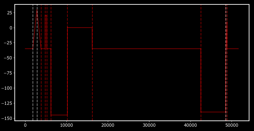
Once we have classified each epoch appropriately, we can run some quality control to clean up any extraneous epochs. I won’t show this, but essentially what it amounts to is a re-iteration of our ‘grouping’ procedure above, but with a larger value than t_avg for the minimum distance between epochs. Lastly, since most people like to work with multiples of 5, we can round our voltages vs to be multiples of 5 as well. The final result should look something like Figure 5, where epochs (dashed lines) corresponding to ramps (blue) and flat steps (red) have been distinguished.

Conclusion

In this post, I tried to describe the why and how for creating and analyzing custom voltage protocols for electrophysiology, specifically within the pClamp software framework. The main advantages of using custom protocols is that any arbitrary waveform can be used as input, circumventing limitations in standard protocol design. However, there are still aspects of protocol design that cannot and/or should not be ignored. For instance, just because you can theoretically specify very large voltages, e.g. Inf, it doesn’t mean you should - patch clamp really only works well when currents are small, and it’s not like the hardware can even deliver arbitrarily large or small voltage commands.

I’ve shown how custom protocols can be created and analyzed, but let me talk briefly about why I think this flexibility can be useful in a practical sense. First, as I’ve mentioned on previous posts, we often want ‘quality control’ steps in our protocols that allow us to estimate quantities such as reversal potentials and conductances. In custom protocols, we can add these epochs within each sweep, or interleave them as separate sweeps. Another important application is that we can specify arbitrarily complex waveforms, such as sinusoids or membrane potentials recorded from live cells. This can be useful in a number of settings, including optimal experimental design or dynamic/action potential clamp experiments.

I hope this post was useful to somebody, but I don’t want to take all the credit for this work. Much of this would not be possible without the monumental respository pyBAF, which is freely available on Github. I strongly encourage every electrophysiologist working in the pClamp ecosystem to check it out. It’s the foundation of a set of tools I’m developing for electrophysiological data curation, analysis, and visualization that I hope to release eventually.

Thank you! As always, comments/feedback are always appreciated.